Model grids
The Basic Model Interface (BMI) supports several different grid types, described below. Depending on the grid type (as returned from the get_grid_type function), a model will implement a different set of grid functions.
Structured grids
For the BMI specification, a structured grid is formed in two dimensions by tiling a domain with quadrilateral cells so that every interior vertex is surrounded by four quadrilaterals. In three dimensions, six-sided polyhedral cells are stacked such that interior vertices are surrounded by eight cells.
In the BMI,
dimensional information is ordered with “ij” indexing
(as opposed to “xy”).
For example,
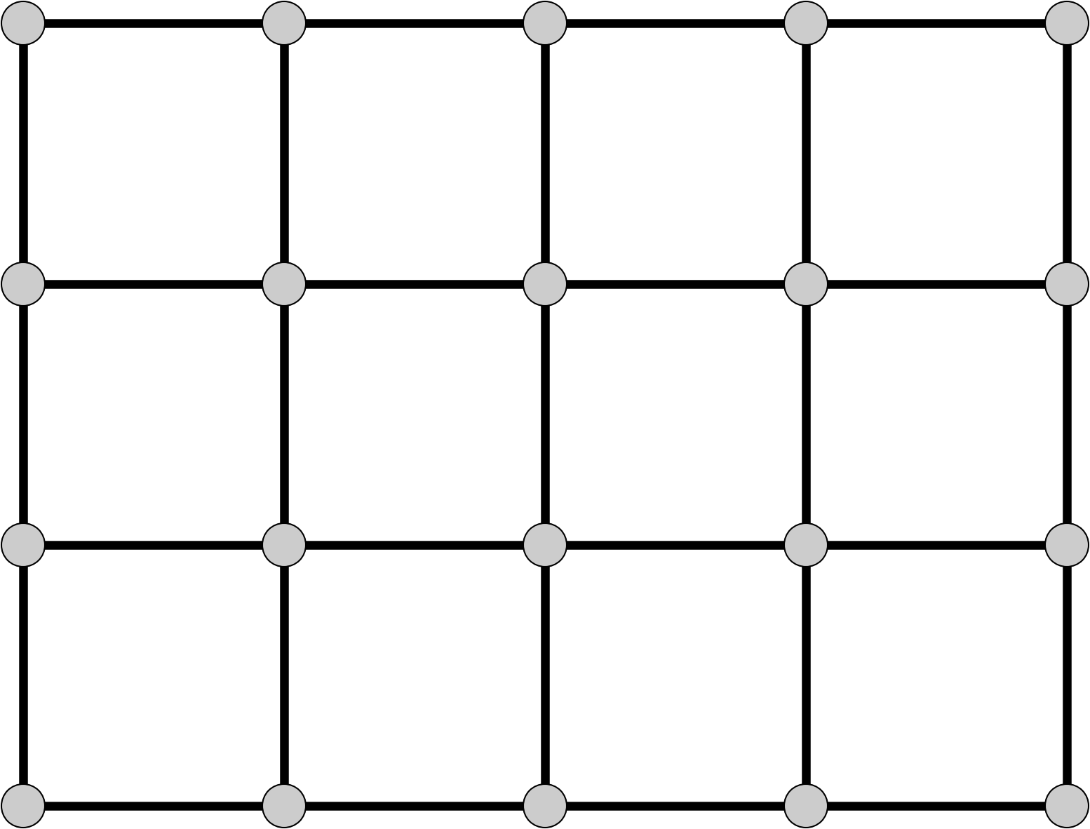
for the uniform rectilinear grid shown below,
the get_grid_shape function would return the array [4, 5].
If there was a third dimension,
its length would be listed first.
Note
The grid shape is the number of rows and columns of nodes, as opposed to other types of element (such as cells or faces). It is possible for grid values to be associated with the nodes or with the cells.
Uniform rectilinear
A uniform rectilinear grid is a special case of structured quadrilateral grid
where the elements have equal width in each dimension.
That is, for a two-dimensional grid, elements have a constant width
of dx in the x-direction and dy in the y-direction.
The case of dx == dy is oftentimes called
a raster or Cartesian grid.
To completely specify a uniform rectilinear grid, only three pieces of information are needed: the number of elements in each dimension, the width of each element (in each dimension), and the location of the corner of the grid.
Uniform rectilinear grids use the following BMI functions:
Rectilinear
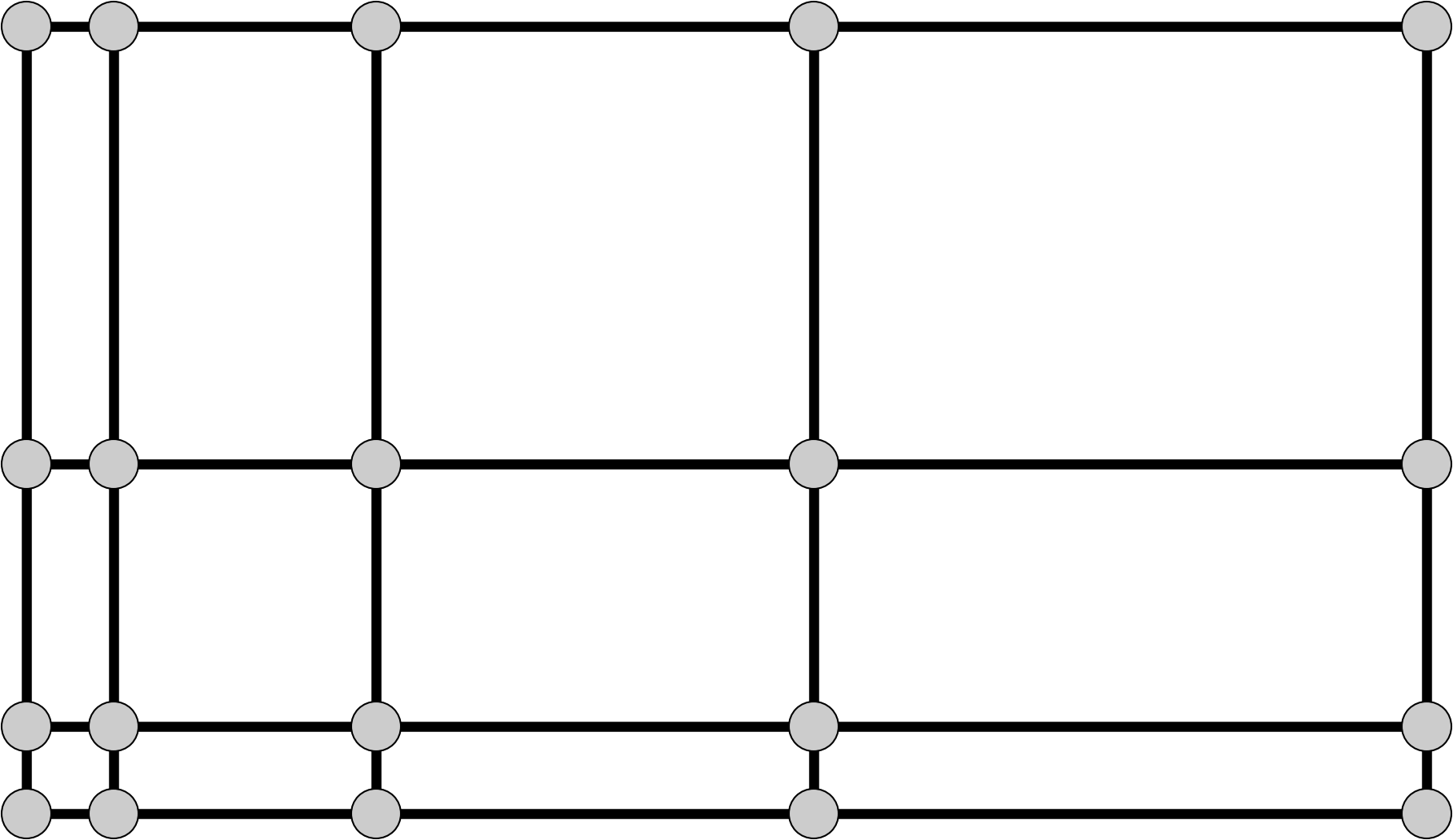
In a rectilinear grid, the spacing between nodes in each dimension varies, as depicted above. Therefore, an array of coordinates for each row and column (for the two-dimensional case) is required.
The get_grid_y function provides an array (whose length is the number of rows, obtained from get_grid_shape) that gives the y-coordinate for each row.
The get_grid_x function provides an array (whose length is the number of columns, obtained from get_grid_shape) that gives the x-coordinate for each column.
Rectilinear grids use the following BMI functions:
Structured quadrilateral
The most general structured quadrilateral grid is one where the rows (and columns) do not share a common coordinate. In this case, coordinates are required for each grid node. For this more general case, get_grid_x and get_grid_y are repurposed to provide this information.
The get_grid_y function returns an array (whose length is the number of total nodes returned by get_grid_size) of y-coordinates.
The get_grid_x function returns an array (whose length is the number of total nodes returned by get_grid_size) of x-coordinates.
Structured quadrilateral grids use the following BMI functions:
Unstructured grids
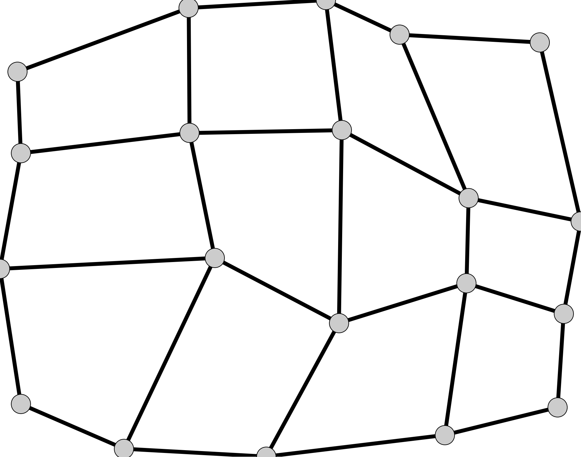
This category includes the unstructured type, as well as the special cases scalar, points, and vector. This is the most general grid type. It can be used for any type of grid. This grid type must be used if the grid consists of cells that are not quadrilaterals; this includes any grid of triangles (e.g. Delaunay triangles and Voronoi tesselations).
Note
A grid of equilateral triangles, while they are most certainly structured, would need to be represented as an unstructured grid. The same is true for a grid of hexagons.
BMI uses the ugrid conventions to define unstructured grids.
Unstructured grids use the following BMI functions:
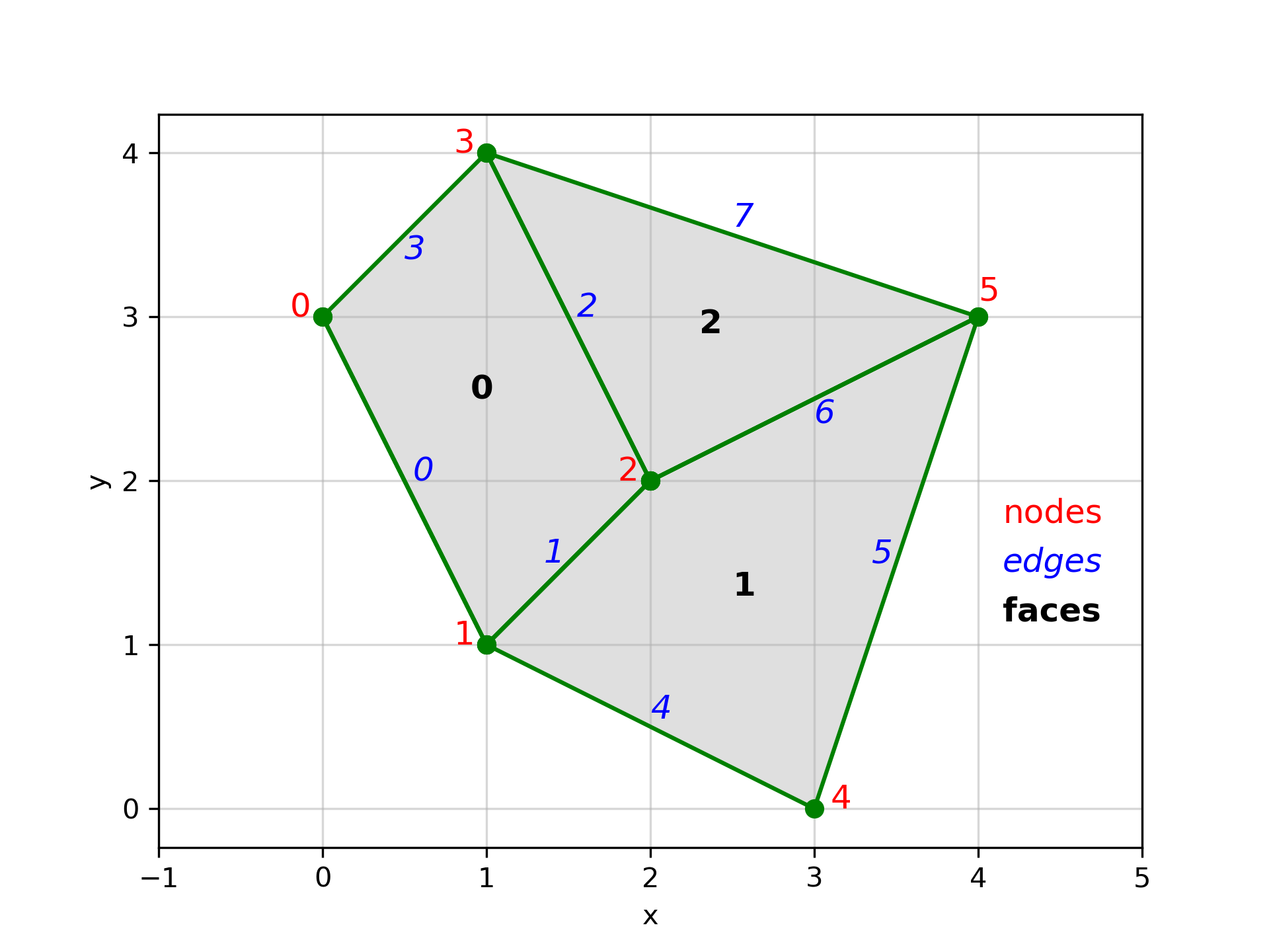
For a demonstration of how these BMI functions work, let’s use the unstructured grid in the annotated figure above.
The grid is two-dimensional, so the get_grid_rank function returns 2.
The nodes of the grid, labeled in the figure in red, are given by coordinates
x = [0, 1, 2, 1, 3, 4]
y = [3, 1, 2, 4, 0, 3]
These will be the outputs of the get_grid_x and get_grid_y functions, respectively. The nodes are indexed, so node 0 is at (x, y) = (0, 3), node 1 is at (x, y) = (1, 1), etc.
As with the grid nodes, the grid edges and faces are indexed. In the figure, the edges are depicted in blue italics, while the faces are boldfaced. The outputs from get_grid_node_count, get_grid_edge_count, and get_grid_face_count are:
node_count = 6
edge_count = 8
face_count = 3
Note that the number of nodes is the length of the x and y vectors above.
The get_grid_nodes_per_face function returns a vector of length face_count. The first two faces are quadrilaterals, while the third is a triangle, so
nodes_per_face = [4, 4, 3]
The get_grid_edge_nodes function returns a vector of length 2*edge_count. The vector is formed, pairwise, by the node index at the tail of the edge, followed by the node index at the head of the edge. For the grid in the figure, this is
edge_nodes = [0, 1, 1, 2, 2, 3, 3, 0, 1, 4, 4, 5, 5, 2, 5, 3]
The get_grid_face_edges function returns a vector of length sum(nodes_per_face). The vector is formed from the edge indices as displayed in the figure:
face_edges = [0, 1, 2, 3, 4, 5, 6, 1, 6, 7, 2]
Likewise, the get_grid_face_nodes function returns a vector of length sum(nodes_per_face). The vector is formed from the node indices as displayed in the figure:
face_nodes = [0, 1, 2, 3, 1, 4, 5, 2, 2, 5, 3]